The two-way ANOVA (analysis of variance) is used to assess the effects of two independent categorical variables (such as gender and college major) – both alone and in combination with each other – on a continuous dependent variable (such as an exam score). In this tutorial we show you how to perform and interpret the results of a two-way ANOVA in SPSS. We also explain how to select follow up tests where these are appropriate.
This tutorial assumes that your study has: (1) a separate sample for each treatment condition or population; and (2) an equal number of participants (or cases) in each group.
Quick Steps
- Click Analyze -> General Linear Model -> Univariate
- Click Reset (recommended)
- Move your dependent variable to the Dependent Variable box
- Move your two independent variables to the Fixed Factor(s) box
- Click Options
- Select Descriptive statistics, Estimates of effect size, and Homogeneity tests
- Click Continue
- Click Plots
- Move the independent variable with the smallest number of levels to the Separate Lines box
- Move the other independent variable to the Horizontal Axis box.
- Click Add
- Click Continue
- Click OK
Assumptions of the Two-Way ANOVA
The assumptions of the two-way ANOVA are:
- The observations in your samples are independent of each other
- The dependent variable is approximately normally distributed in each of the populations from which the samples are drawn. Please see our tutorial on testing for normality in SPSS.
- Homogeneity of variance. Our tutorial includes a test for this assumption.
The Data
Our starting assumption is that you have imported your data into SPSS, and that you’re looking at something like the data set below. (Check out our tutorials on importing data from Excel or MySQL into SPSS).
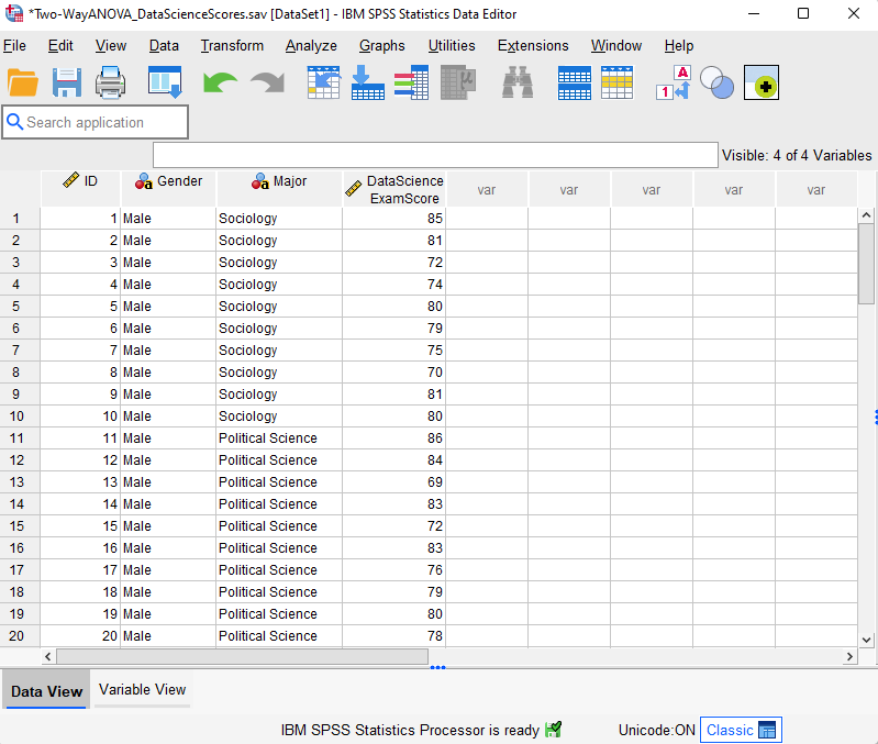
Our fictitious data set contains the Data Science exam scores for 60 students enrolled in one of three majors – Sociology, Political Science, and Economics. We want to know whether these exam scores differ based on students’ gender and major.
Our dependent variable is Data Science exam score.
Our first independent variable (also known as a “factor”) is gender. It has two “levels” – female and male.
Our second independent variable is major. It has three levels – Sociology, Political Science, and Economics.
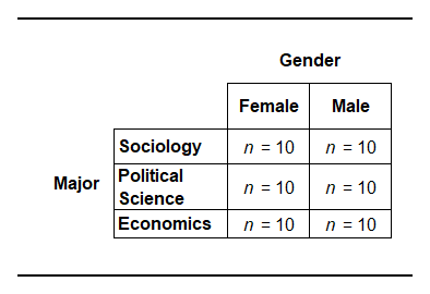
Since gender has two levels and major has three levels, we have six groups of participants (two x three) in our study as illustrated below. There are n = 10 students in each group.
Hypotheses
The two-way ANOVA allows us to evaluate three null hypotheses:
- The main effect for the first independent variable (gender in this example).
H0: There is no difference between the mean Data Science exam scores of male and female students.
- The main effect for the second independent variable (major in this example):
H0: There are no differences between the mean Data Science exam scores for students enrolled in different majors.
- Interaction effect:
H0: There is no interaction effect between gender and major on students’ mean Data Science exam scores
This third hypothesis tests whether the impact of one factor depends on the level of the other factor. For example, does the effect of gender on students’ mean Data Science exam scores depend on their major?
Two-Way Analysis of Variance (ANOVA)
Take the following steps to perform a two-way ANOVA in SPSS.
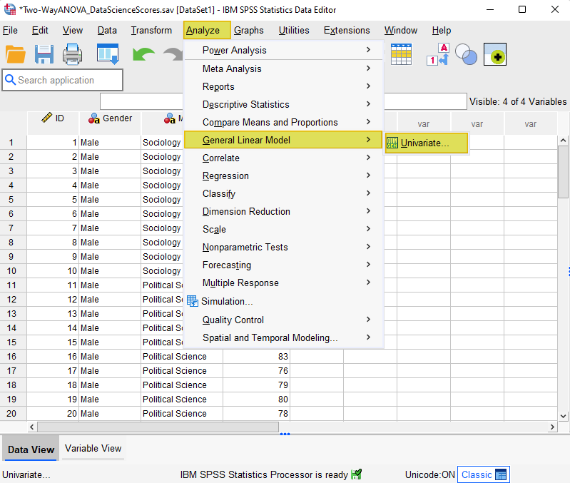
Click Analyze -> General Linear Model -> Univariate as illustrated below.
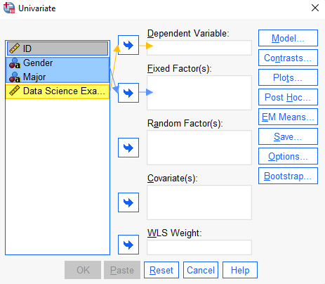
This brings up the Univariate dialog box.
We recommend that you click the Reset button to clear any previous settings.
As per the screenshot below, select your dependent variable (Data Science Exam Score in our example) and use the arrow button to move it to the Dependent Variable box. Then, holding down the CTRL key, select your two independent variables (gender and major in our example) and use the arrow button to move them to the Fixed Factor(s) box.
Select the Options button. This brings up the Univariate: Options dialog box.
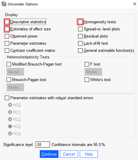
Under Display, select Descriptive statistics, Estimates of effect size, and Homogeneity tests.
Click Continue to return to the Univariate dialog box.
Generate a Profile Plot of Your Group Means
Generating a profile plot (or line graph) of your group means allows you to visualize your data easily, and to assess whether there is an interaction between your two independent variables.
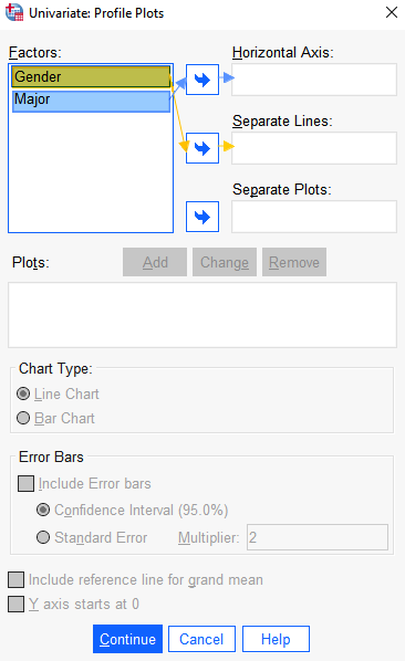
Select the Plots button. This brings up the Univariate: Profile Plots dialog box.
Select one of your independent variables and use the arrow button to move it to the Separate Lines box. Then select the other independent variable and use the arrow button to move it to the Horizontal Axis box. Although you can move either variable to either box, we recommend that you move the variable with the smallest number of levels (gender in our example) to the Separate Lines box.
Click Add. You will see that a plot of your two independent variables (Major*Gender in our example) appears in the Plots box.
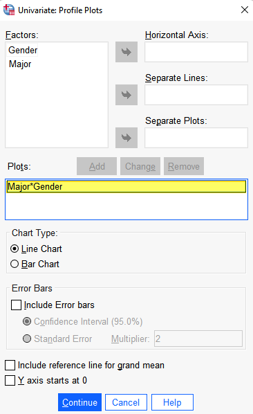
Click Continue to return to the Univariate dialog box.
Click OK.
The SPSS Output Viewer will pop up with the results of your two-way ANOVA.
Check that Homogeneity of Variances Assumption is Met
Once SPSS has generated the results of your two-way ANOVA, the first thing you need to do is to check Levene’s Test of Equality of Error Variances to determine whether your data satisfies the homogeneity of variance assumption of the two-way ANOVA.
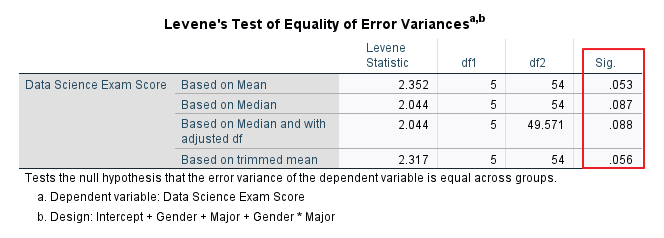
What you want to see is a significance value that is greater than .05. A significance value that is less than .05 would suggest that there are significant differences between the variances of the dependent variable (the Data Science exam scores) across the groups in the study. In our example, none of the values for the Levene’s test is less than .05, so the homogeneity of variance assumption has been met.
Once you have determined that your data satisfies the homogeneity of variance assumption, you can review the Profile Plot (line graph), Tests of Between-Subjects Effects, and Descriptive Statistics.
The two-way ANOVA for the data set described above has a significant interaction effect but, to help you interpret the results of your own two-way ANOVA, we also present the output from a two-way ANOVA for a different fictitious data set that does not have a significant interaction
Results and Interpretation
Results for a Two-Way ANOVA with a Significant Interaction
Reviewing the Profile Plot (line graph) of your group means is the easiest way to get an overview of the results of a two-way ANOVA, and to assess whether there is an interaction between your independent variables. When the lines in your profile plot are clearly not parallel to each other, this indicates that there is a significant interaction effect. When the lines in your profile lot are approximately parallel to each other, this indicates that there is not a significant interaction effect.
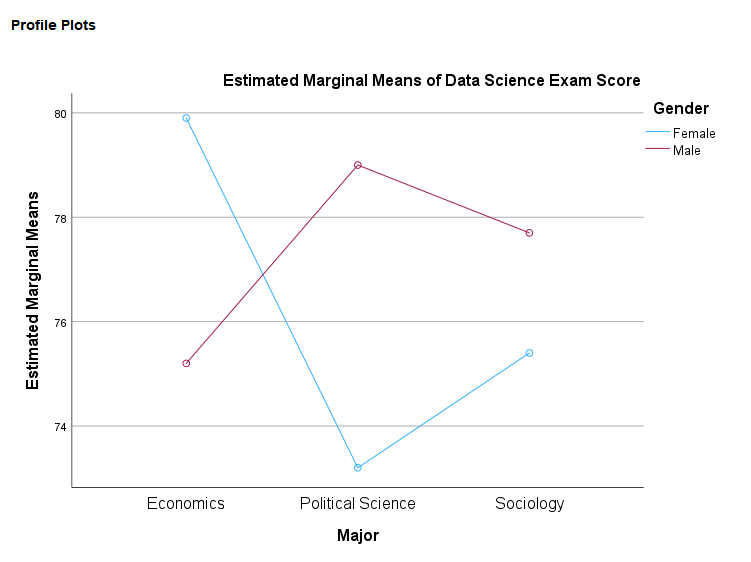
Profile Plot for a Two-Way ANOVA with a Significant Interaction Effect
In the profile plot for our example data set below, it is clear that the lines are not parallel to each other. The mean Data Science exam score for female students in the Economics major is higher than that for male students in the same major. In contrast, the scores for female students are lower than those of their male counterparts in the Political Science and Sociology majors. The differences between male and female scores also vary between majors. There appears to be a significant interaction between gender and major, but we need to review the Tests of Between-Subjects Effects table to confirm this.
Interaction Effect and Main Effects – Example with a Significant Interaction Effect
After you have reviewed your profile plots, the next step is to review the p-values in the “Sig.” column of the Tests of Between-Subjects Effects table to determine whether the interaction effect and/or one or more of the main effects is significant. It is important to determine whether the interaction effect (highlighted in yellow) is significant before considering the main effects (highlighted in blue).
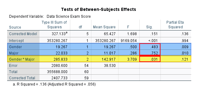
We are using a .05 significance level for this study so the p-value of .031 tells us that the interaction effect between gender and major is significant. This is consistent with the profile plot above. A significant interaction effect means that the effect of one factor depends on the level of the other factor. For example, the effect of gender on student’s Data Science exam score depends on their major. Neither of the p-values for the main effects is significant. It is important to note however, that we should be cautious about interpreting the main effects of a two-way ANOVA when we find a significant interaction effect. In this scenario, it is a good idea to follow up by conducting simple main effects tests to get a gain a better understanding of our data.
The Tests of Between-Subject Effects table also includes the F values and the effect sizes (in the “Partial Eta Squared” column) of the interaction effect and main effects. For example, the F value for the interaction between gender and major is is 3.71 (rounding 3.709 to two decimal places). The effect size is η2 = 0.12 (adding a zero before the decimal point and rounding .121 to two decimal places). We interpret η2 (partial eta squared) as a small effect (0.01), medium effect (0.06), or large effect (0.14) so η2 = 0.12 is a medium effect.
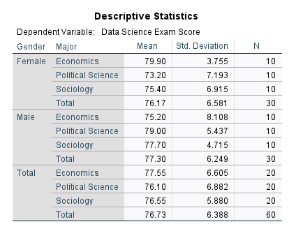
Descriptive Statistics
The Descriptive Statistics table that we requested includes the means and standard deviations for each group in our study.
Results for a Two-Way ANOVA with NO Significant Interaction Effect
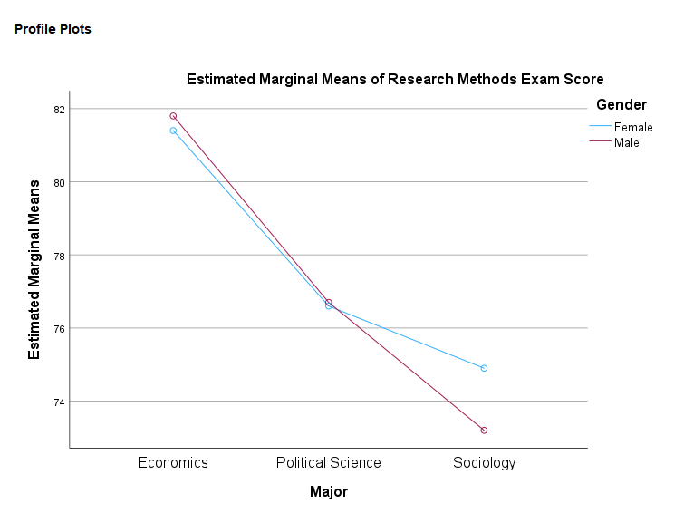
Profile Plot for a Two-Way ANOVA with NO Significant Interaction Effect
The profile plot for our second fictitious study – which aims to find out whether Research Methods exam scores differ based on students’ gender and major – is presented below. In this profile plot, we can see that the lines representing female and male students are approximately parallel to each other. For both female and male students the mean Research Methods exam scores are highest for the Economics major, followed by the Political Science major, and then the Sociology major. There does not appear to be a significant interaction between gender and major. Major appears to have quite a strong effect on students’ Research Methods exam scores but gender appears to have very little effect. Again, we need to review the Tests of Between-Subjects Effects table to learn more about the interaction effect and main effects of his study.
Interaction Effects and Main Effects – Example with NO Significant Interaction Effect
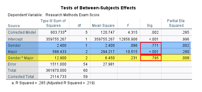
The profile plot above suggests that there is not a significant interaction between gender and major and this is confirmed in the Tests of Between-Subjects Effects table below (interaction effect highlighted in yellow). The p-value .795 is greater than .05, meaning that the interaction effect is not significant.
If you do not find a significant interaction effect, the next step is to determine whether either or both of the main effects is significant. The p-value of .771 for gender is greater than .05 which is not significant. However, the p-value of <.001 for major is lower than .05 which is significant.
If you find a significant main effect for an independent variable with only two levels (such as gender in this study), then you do not need to conduct any further analysis.
However, if you find a significant main effect for an independent variable that has three or more levels (such as major in this example), then the Tests of Between-Subjects Effects table tell us only that there is at least one significant difference among the mean differences for the dependent variable. We don’t know which mean(s) are different from other mean(s). In this scenario, we can follow up by conducting pairwise comparisons to evaluate the differences between each pairing of the levels of the variable (between each pair of majors in this example).
The Tests of Between-Subject Effects table also includes the F values and the effect sizes (in the “Partial Eta Squared” column) of the interaction effect and main effects. For example, the F value for the main effect of major is 10.52 (rounding 10.515 to two decimal places). The effect size is η2 = 0.28 (adding a zero before the decimal point and rounding .280 to two decimal places). We interpret partial eta squared (η2) as a small effect (0.01), medium effect (0.06), or large effect (0.14). Our interaction has a value of η2 = 0.28, so we interpreted this as a large effect.
How to Select an Appropriate Follow Up Test for Your Two-Way ANOVA
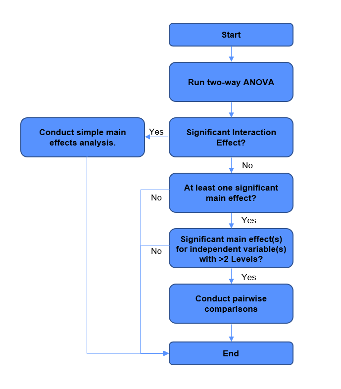
The follow flowchart will help you to select an appropriate follow up test for your two-way ANOVA.
***************
That’s it for this tutorial.
You should now be able to perform a two-way ANOVA in SPSS, check that the homogeneity of variance assumption has been met; interpret your result; and select appropriate follow up tests if applicable.
As noted above, if you found a significant interaction effect between your independent variables, you can follow by up by conducting simple main effects tests.
If you did not find a significant interaction effect between your independent variables, but you found significant main effect(s) for independent variable(s) with more than two levels, you can follow up by conducting pairwise comparisons.
You may also be interested in our tutorials on: (1) reporting the results of a two-way ANOVA in APA style; and (2) exporting your SPSS output to another application such as Word, Excel, or PDF.