In this tutorial we show you how to conduct simple linear regression analysis in SPSS, and interpret the results of your analysis.
Quick Steps
- Visualize your data with a scatterplot
- Click Analyze -> Regression -> Linear
- Move your independent variable to the Independent(s) box
- Move your dependent variable to the Dependent box
- Click Statistics
- Ensure that the Estimates and Model fit boxes are checked
- Place checks in the Confidence intervals and Descriptives boxes
- Place a check in the Durbin-Watson box
- Click Continue
- Click Plots
- Move *ZPRED to the X box.
- Move *ZRESID to the Y box
- Place checks in the Histogram and Normal probability plot boxes.
- Click Continue
- Click OK
The Simple Linear Regression Equation
The goal of simple linear regression is to build a model that will allow us to use the value of one continuous variable (for example a SAT score) to predict the value of another continuous variable (for example a Psychology exam score). The variable that is used to predict another variable is the independent (or predictor) variable. The variable that we want to predict is the dependent (or outcome or criterion) variable.
The regression model is expressed in the form of the following equation:
Ŷ = a + bX
Ŷ = the predicted value of the dependent variable (e.g., Psychology exam score)
a = the y-intercept or constant – the predicted value of the dependent variable (e.g., Psychology exam score) when the independent variable (SAT score) = 0.
Note that a value of 0 is not meaningful for all independent variables. SAT scores, for example, range from 400 to 1600.
b = the slope of the regression line on our scatter plot. The value of b predicts how much our dependent variable (Psychology exam score) changes when our independent variable (SAT score) increases by one unit.
X = the value of the independent variable (e.g., SAT score)
The Data
Our starting assumption for this tutorial is that you have already imported your data into SPSS, and that you’re looking at something like the following:
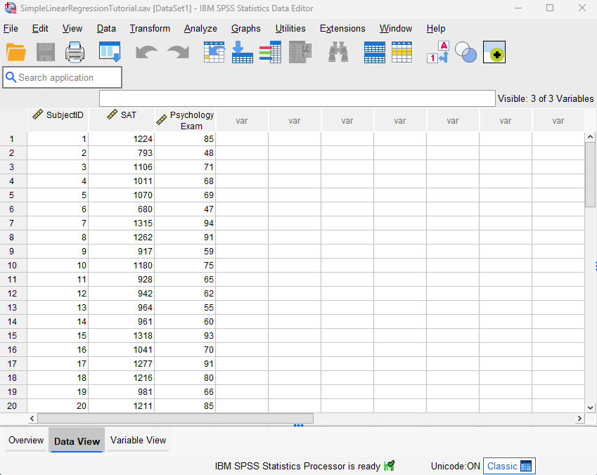
Our fictitious data set contains the SAT scores and Psychology exam scores of 40 students. We want to see if it is possible to use students’ SAT scores to predict their Psychology exam scores.
Assumptions of Simple Linear Regression
There are some assumptions that underlie simple linear regression. These are as follows:
-
- Linearity. There must be a linear relationship between your two variables.
- An absence of extreme outliers. Regression analysis is sensitive to outliers.
- Independence of observations. We usually assume that this assumption is met when the cases (rows) in a data set represent a random sample drawn from a population. Nevertheless, this assumption can be tested in SPSS.
- Normality. The residuals (or errors) of your regression model are approximately normally distributed.
- Homoscedasticity. The variance in the values of your dependent variable (e.g., Psychology exam scores) is similar across all values of your independent variable (e.g., SAT scores).
This tutorial includes steps to check these assumptions in SPSS.
Visualizing Your Data with a Scatterplot
Before you conduct simple linear regression, you should visualize the relationship between your variables to ensure that it is linear. You can do this by creating a scatterplot in SPSS as outlined in our scatterplot tutorial. Move your independent variable (e.g., SAT scores) into the X Axis box, and move your dependent variable (e.g., Psychology exam scores) into the Y Axis box. We also recommend that you add a regression line as outlined in that tutorial. The positive linear relationship between our variables is illustrated below. Negative linear relationships are also appropriate for linear regression analysis. 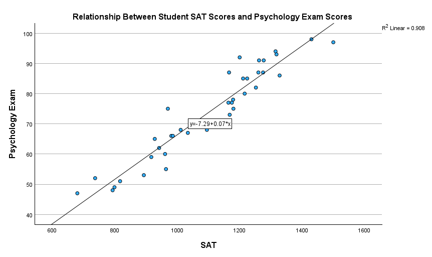
If you don’t see any relationship between your variables, or if you see a non-linear relationship (for example, a curvilinear one), then linear regression analysis isn’t appropriate for your data.
Simple Linear Regression
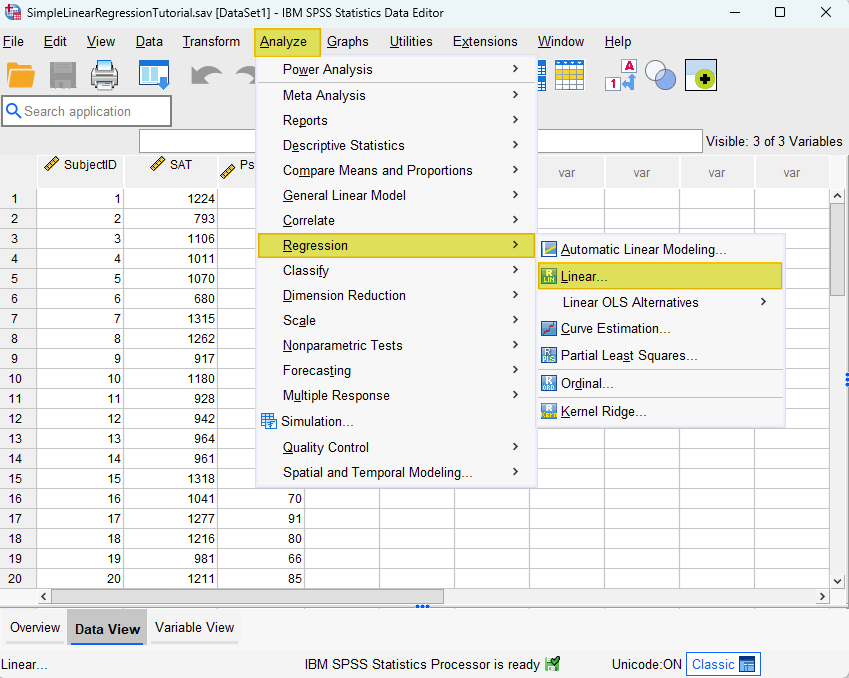
To conduct simple linear regression analysis in SPSS, start by clicking Analyze -> Regression ->Linear as illustrated below.
This brings up the Linear Regression dialog box illustrated below.
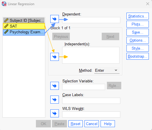
Select your independent/predictor variable (e.g., SAT scores), and use the arrow to move it to Independent(s) box. Then, select your dependent/outcome/criterion variable (e.g., Psychology exam scores) and use the arrow to move it to the Dependent box.
Click the Statistics button. This brings up the Linear Regression: Statistics dialog box.
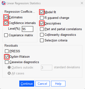
Ensure that the Estimates and Model fit boxes are checked. Next, place checks in the Confidence intervals and Descriptives boxes.
Place a check in the Durbin-Watson box.
Your Linear Regression: Statistics dialog box will now look like the one below:
Click Continue to return to the main Linear Regression dialog box.
Click the Plots button. This brings up the Linear Regression: Plots dialog box illustrated below.
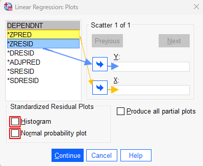
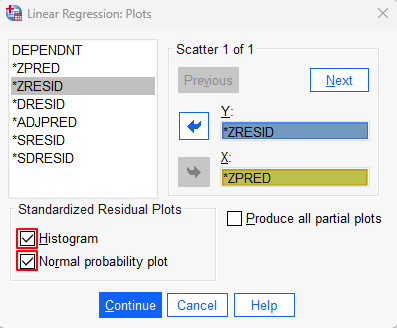
Select *ZPRED and use the arrow button to move it to the X box. Then select *ZRESID and use the arrow button to move to to the Y box.
Check the Histogram and Normal probability plot boxes. Your dialog box should now look as follows:
Click Continue to return to the main Linear Regression dialog box, and then click OK.
The SPSS Output Viewer will pop up with the results of your linear regression analysis and assumption tests.
Check the Assumptions of Simple Linear Regression
We checked the Linearity assumption before we conducted our regression analysis, but now we need to check the remaining assumptions of simple linear regression.
Absence of Extreme Outliers
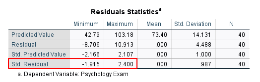
Regression analysis is sensitive to outliers, so we want to ensure that there are no extreme outliers in our data set. We can do this by reviewing the Minimum and Maximum columns of the Std. Residual row in the Residuals Statistics table. A data point with a standardized residual that is more extreme than +/-3 is usually considered to be an outlier. In other words, if the value in the Minimum column of the Std. Residual row is less than -3, we should investigate it. Similarly, if the value in the Maximum column of the Std. Residual row is greater than 3, we should investigate it. Our minimum value of -1.915 and our maximum value of 2.400 indicate that our data set does not include any extreme outliers.
Independence of Observations
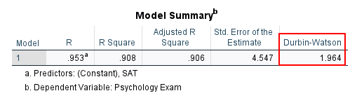
Check the value of the Durbin-Watson statistic in the Model Summary table to determine whether your data satisfies the independence of observations assumption. Values between 1.5 and 2.5 are normally considered to satisfy this assumption. Our value of 1.964 falls well within this range.
Normality
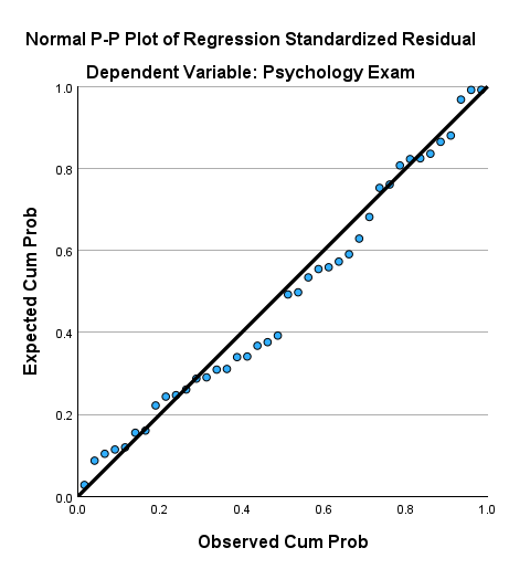
The Normal P-P Plot may be used to test the normality assumption in simple linear regression. This assumption is met if the dots on your P-P Plot are on, or close to, the diagonal line, as in our example below.
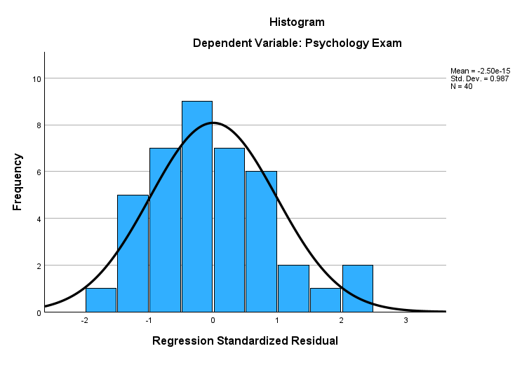
We can also test this assumption by reviewing the histogram of standardized residuals for the dependent variable. If these residuals are approximately normally distributed, as they are in our example below, then the assumption is met.
Homoscedasticity
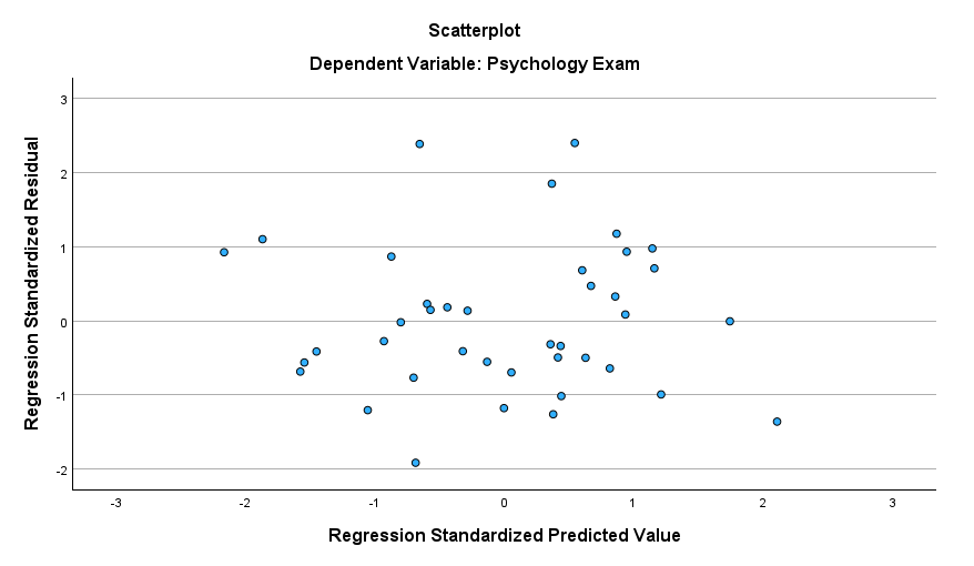
We can check the assumption of homoscedasticity using the scatterplot of standardized residuals versus standardized predicted values. What we want to see is an absence of any pattern. Our fictitious data set satisfies this assumption.
Once we have confirmed that our data satisfies the assumptions of simple linear regression, we are ready to interpret the results of our analysis in the SPSS Output Viewer.
Results and Interpretation
First, we review the Model Summary table. There are several values of interest here:
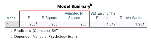
R is the strength of the correlation between our two variables. In our example, there is a very strong correlation of .953 between our SAT and Psychology exam scores. Note that the value of R will always be positive, even when the correlation between the two variables is negative.
R Square tells us how much of the variance in the dependent variable is explained by the independent variable. The value of .908 tells us that 90.8% of the variance in our students’ Psychology exam scores is explained by their SAT scores.
Adjusted R Square adjusts R Square on the basis of our sample size. In our example, the Adjusted R Square of .906 is very similar to the R Square of .908.
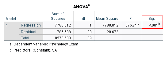
Next, we check the Sig. value in the ANOVA table to determine whether our regression model predicts the dependent variable better than we would expect by chance. Our Sig. value of < .001 is less than .05, indicating that our regression model is significant.
Finally, the Coefficients table gives us the values we need to write the regression equation Ŷ = a + bX. We can then use this equation to predict our dependent variable from our independent variable.
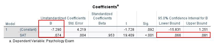
We find the value of a in the (Constant) row of the B column under Unstandardized Coefficients. In our example, this value is -7.290.
We find the value of b in the independent variable row (SAT scores) of the B column under Unstandardized Coefficients. The value of b will be positive, as it is here (.074) when the correlation between your variables is positive. The value of b will be negative when the correlation between your variables is negative.
The regression equation for our example is:
Predicted Psychology exam score = -7.290 + .074(SAT score).
This means that for for every one unit increase in a student’s SAT score, we predict that their Psychology exam score will increase by .074 units. Using this equation, we would predict that a student with a SAT score of 1100 would have a Psychology exam score of 74.11 as follows:
Predicted Psychology exam score = -7.290 + .074(1100) = 74.11
The 95.0% Confidence Interval for B in the row for your independent variable (e.g., SAT scores) indicates that we can be 95% confident that the population value for the slope of the regression line between our variables lies between .66 and .81.
Additional Considerations
Even if your regression model is significant, there are some additional considerations to keep in mind when interpreting the results of simple linear regression analysis:
- Linear regression doesn’t prove causation: a statistically significant regression model doesn’t prove that a cause-and-effect relationship exists between two variables. We cannot, for example, use our regression equation to say that an increase in SAT scores causes an increase in Psychology exam scores.
- Extrapolation: You should use your regression model to predict dependent variable values only for values of the independent variable that fall within the range that you used to create your regression equation. In our data set, the lowest and highest SAT scores are 680 and 1500 respectively. Thus, we should not use it to predict a Psychology exam score for a student with a SAT score of 420, for example, because that score is outside the range of values used to create our regression equation.
- The Limits of Prediction with One Independent Variable: Simple linear regression uses only one independent variable to predict a dependent variable. In reality, however, social phenomena are often related to many other variables. In many cases, a regression model that combines two or more independent variables – as multiple regression does – may predict a dependent variable more accurately than does a simple linear regression model. For example, it is possible that a regression model that includes both SAT scores and the amount of time spent studying for the exam might predict Psychology exam scores more accurately than SAT scores alone.
***************
That’s it for this tutorial. You should now be able to conduct simple linear regression analysis in SPSS, and interpret the results of your analysis. You may also be interested in our tutorial on reporting simple linear regression from SPSS in APA style.
***************