In this tutorial, we show you how to report the results of a repeated-measures ANOVA from SPSS in APA style. First, we give you a template that you can use for this purpose. Then, we show you how to populate this template using your own SPSS output. Finally, we provide an example of a repeated-measures ANOVA report written using our template.
For more general information about formatting your reports in APA style, please refer to the APA Style website.
Template for Reporting a Repeated-Measures ANOVA in APA Style
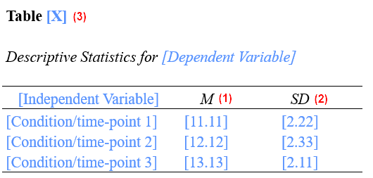
A template for reporting your repeated-measures ANOVA is below. Replace the [blue text in square brackets] with information from your own ANOVA. The (red numbers in parentheses) correspond to the numbers on screenshots of SPSS output and to our notes for writing your report (see below).
APA Template Text
A repeated-measures ANOVA was performed to evaluate the effect of [independent variable] on [dependent variable]. The means (1) and standard deviations (2) for [dependent variable] are presented in Table [table number] (3).
(4) Mauchly’s test indicated that the assumption of sphericity had been [met/violated] (5), χ2 ([Mauchly’s test df]) (6) = [Aprox. Chi-Square for Mauchly’s test] (7), p = [Mauchly’s test p value] (8), (9) and therefore degrees of freedom were corrected using [Greenhouse-Geisser/Huynh-Feldt] (10) estimates of sphericity (ε = [ε value] (11)). The effect of [independent variable] on [dependent variable] [was/was not] (12) significant at the [alpha level] (13) level, F([independent variable df ] (14), [error df]) (15) = [F value] (16), p = [p value] (17), partial η2 = [partial η2 value] (18).
Note: Include the following section only if your ANOVA was significant.
Post-hoc pairwise comparisons with a [name of adjustment for multiple comparisons] (19) adjustment indicated that (20) there was no significant difference between the [dependent variable] at [level A of independent variable] and [level B of independent variable], (p = [p value] (21)) and/or (22) [dependent variable] was significantly [higher/lower] (23) at [level B of independent variable] than at [level A of independent variable], (p = [p value] (24)).
Populating the APA Template With Your SPSS Output
The screenshots of SPSS output below are from a repeated-measures ANOVA that we performed (on data from a hypothetical study) evaluating the effect of time on untreated fear of spiders as measured by SPQ scores. The numbers on these screenshots refer to numbers in the APA reporting template above. Use the corresponding values from your own SPSS output to populate our template.
The APA Style Guide states: (a) that the first line of each paragraph should be indented 0.5 inches from the left margin; and (b) that the text should be double-spaced.
We encourage you to modify the wording of the template as needed for your own ANOVA, and to ensure that your report is clear and easy to understand.
Important: p values are reported for: Mauchly’s test; the repeated-measures ANOVA itself; and (if applicable) post-hoc tests. Be sure to use the correct p value(s) in each case as described below.
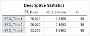
(1) Report the means to two decimal places.
(2) Report the standard deviations to two decimal places.
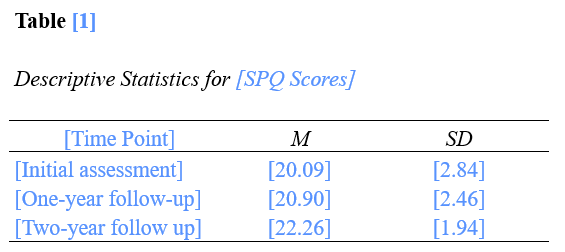
(3) You need to number the tables in APA reports. If this is the first table in your report, it will be Table 1. See our tutorial on formatting SPSS tables in APA style. The means and standard deviations can be included in the text instead, but they are often easier to read when they are presented in a table.
Mauchly’s Test (Optional)
(4) We recommend reporting the results of Mauchly’s Test of Sphericity since sphericity is an assumption of the repeated-measures ANOVA. You can use the template text highlighted in grey to do so. If sphericity is violated, you will also need the text highlighted in green as described in (9) below.
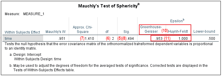
(5) Use the p value in the “Sig.” column of the “Mauchly’s Test of Sphericity” table to determine whether the assumption of sphericity is met or violated:
- This assumption is met if the p value in the “Sig.” column of the this table is greater than .05 (i.e., not significant). As illustrated above, the Mauchly’s test p value of .494 for our hypothetical study is greater than .05, so this assumption is met in this case.
- This assumption is violated if the p value in the “Sig.” column of the this table is less than or equal to .05 (i.e., significant).
(6) Report the degrees of freedom (df) from the df column of your Mauchly’s test table.
(7) Report the χ2 value as per the “Approx Chi-Square” volumn of your Mauchly’s test table to two decimal places.
(8) Report the exact Mauchly’s test p value to two or three decimal places. However, if the p value is .000, report it as < .001. Do not add a leading zero to your p value.
(9) If you have reported the results of Mauchly’s test, and the assumption of sphericity is violated, you will need to include the text highlighted in green. This text is not applicable if the assumption of sphericity is met.
(10) When the assumption of sphericity is violated, use the Greenhouse-Geisser or Huynh-Feldt estimates of sphericity to correct the degrees of freedom when you report your repeated-measures ANOVA. In general, the guideline is:
- If the Greenhouse-Geisser epsilon (ε) is less than than .75, use the Greenhouse-Geisser estimate of sphericity
- If the Greenhouse-Geisser epsilon (ε) is greater than .75, use the Huynh-Feldt estimate of sphericity
(11) Report the relevant epsilon above) to two decimal places.
Repeated-Measures ANOVA
You will find the values that you need to report for the repeated-measures ANOVA in the “Tests of Within-Subjects Effects” table as illustrated below. Select the relevant values from your SPSS output as follows:
- Use the values for “Sphericity Assumed” if your data meets the assumption of sphericity as described in (5) above.
- Use the values for “Greenhouse-Geisser” if your data violates the assumption of sphericity and the epsilon (ε) for Greenhouse-Geisser in the “Mauchly’s Test of Sphericity” table is less than than .75.
- Use the values for “Huynh-Feldt” if your data violates the assumption of sphericity and the epsilon (ε) for Greenhouse-Geisser in the “Mauchly’s Test of Sphericity” table is greater than .75.
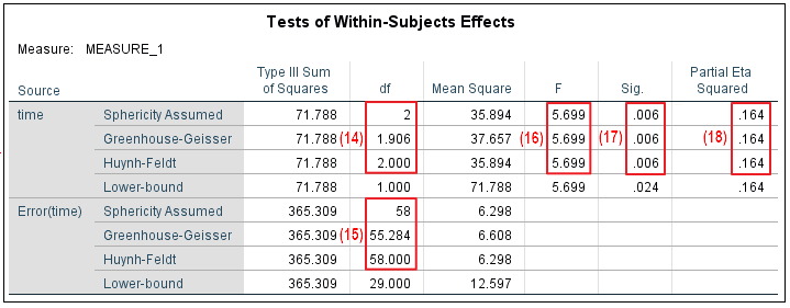
(12) Your repeated-measures ANOVA is significant if the p value listed in the relevant row of othe “Sig.” volumn of the “Tests of Within-Subjects Effects” table (see point (17)) is less than or equal to the alpha level you selected for your ANOVA as reported in (13).
(13) Select an alpha level before you conduct your ANOVA. An alpha level of .05 is typical.
(14) Report the relevant df for the independent variable as per the top section of the table. This refers to the between groups df.
(15) Report the relevant df for the error as per the bottom section of the table. This refers to the within groups df.
(16) Report the relevant F value from the SPSS output to two decimal places. Add a leading zero to your F value if it is less than 1.00 (for example an F value of .791 would be reported as 0.79).
(17) Report the exact p value to two or three decimal places as per the “Sig.” column of the “Tests of Between-Subjects Effects” table. However, if the p value is .000, report it as < .001. Do not add a leading zero to your p value.
(18) Report the partial η2 value to two decimal places. You should not add leading zeros to this value. If you have a partial η2 of less than .005, we suggest reporting this as < .01 rather than rounding it down to .00
Post-Hoc Tests
You should only include the text in this section of the report if your ANOVA was significant as per (12) above. You will find most of the information you need in the “Pairwise Comparisons” table in your SPSS output. Note that this table duplicates each pairwise comparison (e.g., there are six rows in our table although there are only three pairwise comparisons).
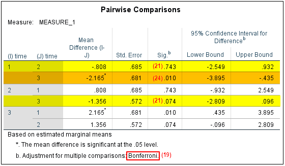
(19) The name of the adjustment used is stated in the notes beneath the “Pairwise Comparisons” table as illustrated in the screenshot above.
(20) Use the text highlighted in yellow to report any pairwise comparisons that were not significant. Pairwise comparisons are not significant if the p value in the “Sig.” column is greater than the alpha level that you selected for the comparisons (SPSS has a default alpha level of .05). In our example, there were no significant differences: (1) between the SPQ scores at the initial assessment and at the one-year assessment (i.e., between time 1 and time 2); or (2) between the SPQ scores at the one-year assessment and at the two-year assessments (i.e., between time 2 and time 3). We have highlighted these non-significant comparisons in yellow in our example table.
Although we have reported the non significant pairwise comparisons first, you can report the significant comparisons first if this makes more sense for your own study.
(21) Report the exact p value for each non-significant pairwise comparison to two or three decimal places as per the “Sig.” column of the “Pairwise Comparisons” table. As noted earlier, you should not add leading zeros to your p values.
(22) Use the text highlighted in gold to report any pairwise comparisons that were significant. Pairwise comparisons are significant if the p value in the “Sig.” column is less than or equal to the alpha level selected for the comparisons (SPSS uses a default alpha level of .05). SPSS adds an asterisk to the value in the “Mean Difference (I-J)” column for differences that are significant. In our example, there was a significant difference between the SPQ scores at the initial assessment and those at the two-year assessment (i.e., between time 1 and time 3). We have highlighted this comparison in gold in the table above.
(23) The easiest way to determine whether the dependent variable (e.g., SPQ scores) for one level of an indepent variable (e.g., time) is higher or lower than for another level of that independent variable is to review the “Mean” column of the “Descriptive Statistics” table. In our example, we can see that the SPQ scores are higher at time 3 (the two-year assessment) than at time 1 (the initial assessment).
You may also wish to consider using adjectives other than higher/lower to describe these differences, for example, greater/smaller.
(24) Report the exact p value for each significant pairwise comparison to two or three decimal places as per the “Sig.” column of the “Pairwise Comparisons” table. However, if the p value is .000, report it as < .001. As noted previously, you should not add leading zeros to your p values.
Example of a Repeated-Measures ANOVA Report in APA Style
A repeated-measures ANOVA was performed to evaluate the effect of [time] on [untreated fear of spiders as measured on the SPQ scale]. The means and standard deviations for [the SPQ scores] are presented in Table [1].
Mauchly’s test indicated that the assumption of sphericity had been [met], χ2 ([2]) = [1.41], p = [.494]. The effect of [time] on [untreated fear of spiders] [was] significant at the [.05] level, F([2], [58]) = [5.70], p = [.006], partial η2 = [.16].
Post-hoc pairwise comparisons with a [Bonferroni] adjustment indicated that there was no significant difference between the [SPQ scores] at [the initial assessment] and [at the follow-up assessment one year later], (p = [.743]). Similarly, there was no significant difference between the [SPQ scores] at [the one-year] and [two-year follow up assessments], (p = [.074]). However, [SPQ scores] was significantly [higher] at [the two-year follow-up assessment] than at [the initial assessment], (p = [.010]).
***************
That’s it for this tutorial. You should now be able to report a repeated-measures ANOVA and post-hoc tesing performed in SPSS in APA style.
***************