In this tutorial, we’ll look at how to conduct the Mann-Whitney U Test in SPSS, and also at how to interpret the result of the test.
The Mann-Whitney U Test evaluates whether two samples are likely to originate from the same underlying population, and it tends to be used in situations where an independent-samples t test is not appropriate (for example, if either of the sample distributions are non-normal).
Quick Steps
- Click Analyze -> Nonparametric Tests -> Legacy Dialogs -> 2 Independent Samples.
- Drag and drop the dependent variable into the Test Variable(s) box, and the grouping variable into the Grouping Variable box.
- Tick Mann-Whitney U under Test Type.
- Click on Define Groups, and input the values that define each of the groups that make up the grouping variable (i.e., the coded value for Group 1 and the coded value for Group 2).
- Press Continue, and then click on OK to run the test.
- The result will appear in the SPSS data viewer.
For this tutorial, we’re using data from a fake study that looks at the relationship between dog ownership and the ability to throw a frisbee.
The Data
As per usual, we’re working on the assumption that you’ve opened SPSS, you’re looking at the Data View, and it looks something like this.
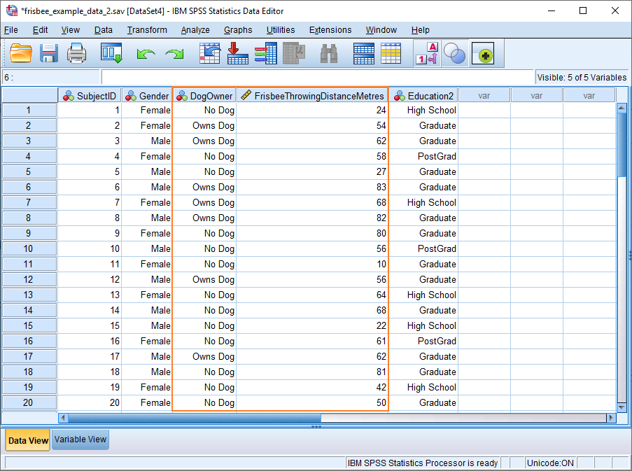
In our example, Frisbee Throwing Distance in Metres is the dependent variable, and Dog Owner is the grouping variable. Put simply, we want to know whether owning a dog (independent variable) has any effect on the ability to throw a frisbee (dependent variable).
Assumption of Normality
Given this setup, it would be usual to conduct an independent samples t test. One assumption of this parametric test is that data is normally distributed. The trouble is if we test our data for normality, we get this result.
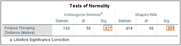
Both Kolmogorov-Smirnov and Shapiro-Wilk suggest that our dependent variable is not distributed normally. This is confirmed by the histogram, which has a long left tail.
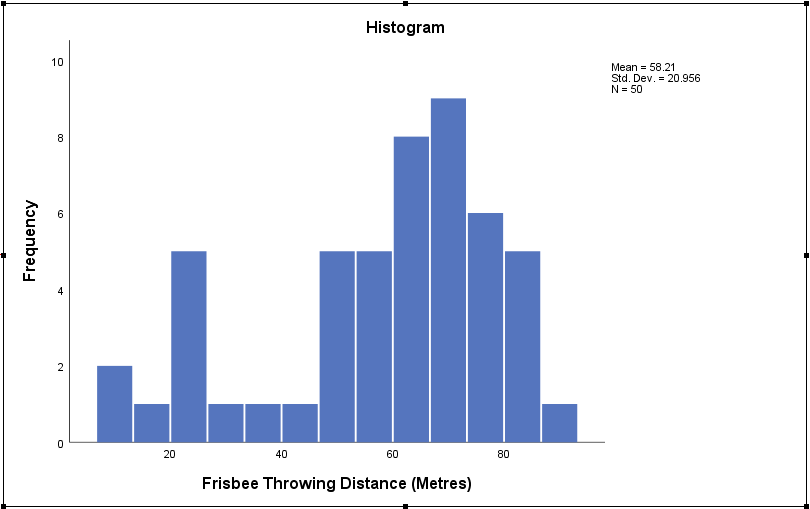
This means we’re better off using a non-parametric test to determine whether there is a relationship between our independent and dependent variables (though, actually, since we have a large number of observations, we’d probably get away with the t test). The obvious choice here is the Mann-Whitney U test.
Mann-Whitney U Test
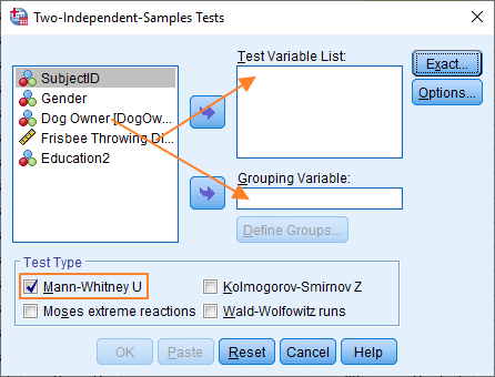
To begin, click Analyze -> Nonparametric Tests -> Legacy Dialogs -> 2 Independent Samples. This will bring up the Two-Independent-Samples Tests dialog box.
The setup here is not too difficult.
To perform the Mann-Whitney U test, we’ve got to get our dependent variable (Frisbee Throwing Distance) into the Test Variable List box, and our grouping variable (Dog Owner) into the Grouping Variable box. To move the variables over, you can either drag and drop, or use the blue arrows.
You also need to select Mann-Whitney U under Test Type (by ticking the box).
The dialog should now look something like this.
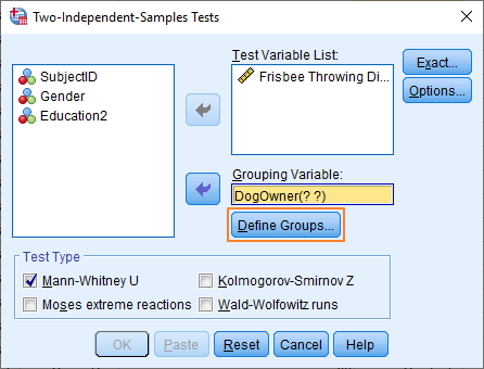
You’ll notice that the Grouping Variable, DogOwner, has two question marks in brackets after it. This indicates that you need to define the groups that make up the grouping variable. Click on the Define Groups button.
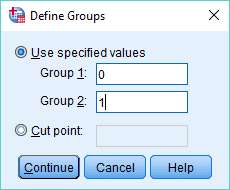
We’re using 0 and 1 to specify each group, because these values match the way the variable is coded (the Data View shows value labels, not the underlying numeric values). 0 is No Dog; and 1 is Owns Dog.
It’s also worth noting that if you had coded your grouping variable as a String type, then you’d need to match the string values that appear in the Data View precisely – for example, “No Dog” and “Owns Dog”.
Once you have specified the values that define each group, press the Continue button, and then click on OK in the main dialog box to run the Mann-Whitney U test.
The Result
The result will appear in the SPSS Output Viewer.
The Mann-Whitney test works by converting scores into ranks while ignoring the grouping variable (in our example, ownership and non-ownership of a dog), and then comparing the mean rank of each group. If the difference between the mean ranks is big enough to be significant, then the null hypothesis that the samples derive from the same population is rejected.
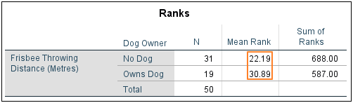
As you can see above, there is what looks like a sizeable difference between the mean ranks of the No Dog and Owns Dog groups. The Mann-Whitney test statistic will tell us whether this difference is big enough to reach significance.
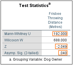
SPSS produces a test statistics table to summarise the result of the Mann-Whitney U test. The key values are Mann-Whitney U, Z and the 2-tailed significance score.
In our example, the No Dog group comprises greater than 20 observations. This means we can use the value of Z to derive our p-value. Otherwise, the significance value comes from U.
SPSS is reporting a Z score of -2.049 and a 2-tailed p-value of .040. This would normally be considered a significant result (the standard alpha level is .05). Therefore, we can be confident in rejecting the null hypothesis that holds that the Owns Dog and No Dog groups are drawn from the same underlying population. Or, to put this another way, the result of the Mann-Whitney U test supports the proposition that owners and non-owners of dogs have different frisbee throwing abilities.
***************
Okay, that’s the end of this tutorial. You should now have a good idea of how to perform the Mann-Whitney U test in SPSS, and how to interpret the result. You may also be interested in our tutorials on: (1) exporting your SPSS output to another application such as Word, Excel, or PDF and (2) reporting Mann-Whitney U test results from SPSS in APA style.