This quick tutorial will show you how to interpret the result of a chi square calculation you have performed in SPSS.
The Result
The tutorial starts from the assumption that you have already calculated the chi square (test of independence) statistic for your data set, and you want to know how to interpret the result that SPSS has generated. (We have a different tutorial explaining how to do a chi square test in SPSS).
You should be looking at a result that looks something like this in the SPSS output viewer.
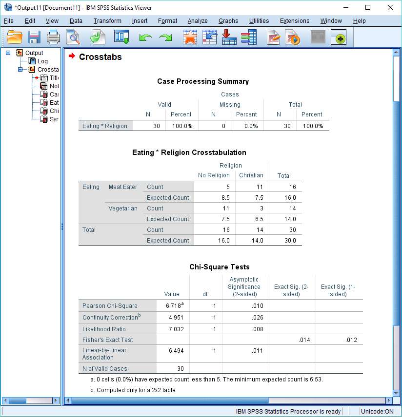
The crosstabs analysis above is for two categorical variables, Religion and Eating. Each variable has two possible values: No Religion and Christian for the Religion variable; Meat Eater and Vegetarian for the Eating variable.
The null hypothesis of our hypothetical study is that these variables are not associated with each other – they are independent variables. The chi square test allows us to test this hypothesis.
The output of a crosstabs analysis contains a number of elements. Let’s look at each in turn.
Case Processing Summary
As its name suggests, the Case Processing Summary is just a summary of the cases that were processed when the crosstabs analysis ran.
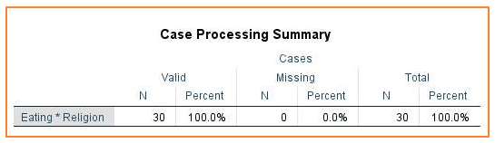
In our example, as you can see above, we had 30 valid cases, and no missing cases.
Eating * Religion Crosstabulation
This is the crosstabs table, and it provides a lot of information that is useful for interpreting a chi square test result.
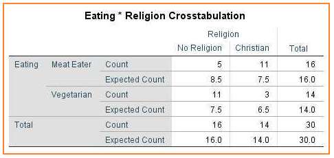
Our crosstabs table includes information about observed counts (what SPSS calls “Count”) and expected counts.
Observed Count
The observed count is the observed frequency in a particular cell of the crosstabs table. For example, our table shows that 5 meat eaters (out of a total of 16) have no religion and 3 Christians (out of a total of 14) are vegetarian.
Expected Count
The expected count is the predicted frequency for a cell under the assumption that the null hypothesis is true. In our case, the null hypothesis is that there is no association between the Eating variable and the Religion variable, which means the expected count is the predicted frequency for a cell on the assumption that eating and religion are not dependent on each other.
Importance of Observed and Expected Counts
If you want to understand the result of a chi square test, you’ve got to pay close attention to the observed and expected counts. Put simply, the more these values diverge from each other, the higher the chi square score, the more likely it is to be significant, and the more likely it is we’ll reject the null hypothesis and conclude the variables are associated with each other.
If you look at the crosstabs table above, you’ll see that there are more Christian meat eaters than would be expected were the null hypothesis (that the variables are independent) true; and fewer Christian vegetarians. And similarly, there are more atheist vegetarians than would be expected, and fewer atheist meat eaters.
The question is whether these differences are big enough to allow us to conclude that the Eating variable and Religion variable are associated with each other. This is where the chi square statistic comes into play.
Chi-Square Tests
As you can see below, SPSS calculates a number of different measures of association.
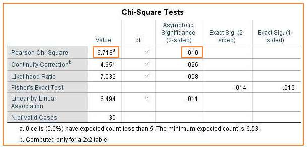
We’re interested in the Pearson Chi-Square measure.
The chi square statistic appears in the Value column immediately to the right of “Pearson Chi-Square”. In this example, the value of the chi square statistic is 6.718.
The p-value (.010) appears in the same row in the “Asymptotic Significance (2-sided)” column. The result is significant if this value is equal to or less than the designated alpha level (normally .05). In this case, the p-value is smaller than the standard alpha value, so we’d reject the null hypothesis that asserts the two variables are independent of each other. To put it simply, the result is significant – the data suggests that the variables Religion and Eating are associated with each other.
The chi square statistic only tells you whether variables are associated. If you want to find out how they are associated then you need to return to the crosstabs table. In our example, the crosstabs table tells us that atheism is disproportionately associated with vegetarianism and meat eating is disproportionately associated with Christianity.
***************
That’s all for this tutorial. You should now have a good idea of how to interpret chi square results in SPSS. Check out our tutorial on reporting Chi Square results from SPSS in APA format.
***************
EZSPSS on YouTube
The second half of our SPSS chi square video includes a discussion of how to interpret chi square results in SPSS.