In this tutorial, we show you how to calculate a minimum sample size for a Pearson correlation coefficient using SPSS power analysis. It is important to perform this calculation before you collect data for your study (although you may wish to carry out a pilot study beforehand).
Quick Steps
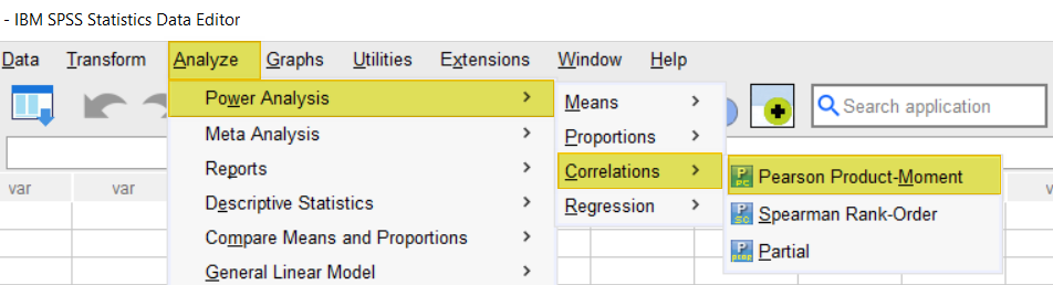
- Click Analyze -> Power Analysis -> Correlations -> Pearson Product Moment
- Click Reset (recommended)
- For Estimate, ensure that Sample size is selected
- In the Single power value box, enter your desired power value (typically .80 or higher)
- In the Pearson correlation parameter box, enter the expected correlation between your variables of interest
- In the Null value box, you will typically leave the value as 0
- Ensure that the Use bias-correction formula in the power estimate box is checked
- Under Test direction, select Nondirectional (two-sided) analysis or Directional (one-sided) analysis as applicable
- In the Significance level box, overtype the default value of 0.05 if applicable
- Click OK
What do we Need to Calculate Sample Size for a Pearson Correlation?
Imagine that we want to conduct a study to find out whether there is an association between the scores that students receive on their Spanish language exam and the number of minutes that they report studying for the exam. We plan to collect data from a sample of students, and then calculate a Pearson correlation coefficient to analyze this data. Before we collect any data, however, we want to estimate the minimum sample size that we need for our study.
To calculate the minimum sample size for a Pearson correlation test, we need the following:
- the power value
- the expected correlation between the variables of interest
- the correlation for the null hypothesis
- a decision about whether the alternative hypothesis is directional or non-directional
- the alpha level
Power Value
Power refers to the probability that a statistical test will detect an effect, difference, or correlation if that effect, difference, or correlation exists. If the test does not detect an effect when an effect does, in fact, exist, researchers will incorrectly fail to reject the null hypothesis, thereby committing a Type II error.
The standard convention is to use a power value of .80 (or higher). This means that we will detect a statistically significant effect 80% of the time if an effect exists.
In our example, this means that a Pearson correlation coefficient test will detect a significant correlation between students’ Spanish language exam scores and the number of minutes they report studying for the exam 80% of the time if these two variables are, in fact, correlated.
If all the other factors used to calculate sample size are held constant, the higher the power value, the larger the minimum sample size.
Expected Correlation Between the Variables of Interest
We need an estimate of the expected correlation between the two variables of interest. That is, we need to know the expected r value. You can base this estimate on: a pilot study; or one or more previous studies that are similar to yours.
If you can’t run a pilot study, and there are no previous studies that are similar to yours, however, you can use Cohen’s (1988) effect size recommendations to make an educated guess about the likely correlation coefficient between your variables: r = .10 (small effect), r = .30 (medium effect), and r = .50 (large effect)
For our example, we will use r = .34 based on the findings of a previous (fictitious) study that was similar to ours.
If all the other factors used to calculate sample size are held constant, the higher the expected correlation for the variables of interest, the smaller the minimum sample size.
Correlation for the Null Hypothesis
When we calculate a minimum sample size, we need to enter a correlation coefficient for our null hypothesis. For most studies, the null hypothesis is that there is no correlation between the variables of interest (r = .00).
Directional or Non-Directional Alternative Hypothesis?
You will need to determine whether the alternative hypothesis for your study is directional (one-tailed) or non-directional (two-tailed). Since a previous study that was very similar to ours found a positive correlation between these two variables, we have opted for a directional hypothesis as follows:
- Students’ Spanish language exam scores are positively correlated with the number of minutes that they report studying for the exam (the more time they report studying for the exam, the higher their score).
If you cannot justify a directional hypothesis, you should use a non-directional hypothesis.
If all the other factors used to calculate sample size are held constant, you will need a larger sample size for a non-directional hypothesis than for a directional hypothesis.
Alpha Level
The alpha level (also known as the significance level or p value) refers to the probability that a statistical test will find an effect, difference, or correlation when, in fact, that effect, difference, or correlation does not exist. In other words, it is the probability that we will incorrectly reject the null hypothesis, thereby committing a Type I error.
The standard convention is to set the alpha level at .05 (or less), which means that there is a 5% probability that we will reject the null hypothesis when, in fact, that effect, difference, or correlation does not exist.
If all the other factors used to calculate sample size are held constant, the lower the alpha level, the larger the minimum sample size.
Calculating Sample Size for a Pearson Correlation Using SPSS Power Analysis
To calculate a sample size for a Pearson Correlation, first click Analyze -> Power Analysis -> Correlations -> Pearson Product Moment
This brings up the Power Analysis: Pearson Correlation dialog box.
We recommend clicking the Reset button to clear any previous settings.
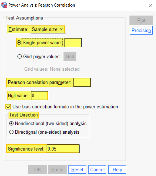
Under Test Assumptions, for Estimate, ensure that Sample size is selected.
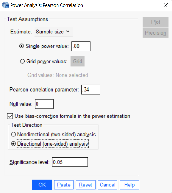
Then, in the Single power value box, enter your desired power value. For our example, we will enter .80 following the standard convention.
In the Pearson correlation parameter box, enter the expected correlation between your variables of interest. We enter a value of .34 on the basis of a previous (fictitious) study that was similar to ours.
In the Null value box, we leave the default value of 0 unchanged. We rarely need to change this.
Ensure that the Use-bias correction formula in the power estimate box is checked.
Under Test direction, the Nondirectional (two-sided) analysis option is selected by default. You should only select the Directional (one-sided) analysis option if you can justify this decision. In our example, we select the the Directional (one-sided) analysis option on the basis of the results of a previous similar (fictitious) study.
By default, the Significance level box is set to a value of 0.05. if you intend to use an alpha level other than .05, overtype this value with your chosen alpha level.
The screenshot below shows the Power Analysis: Pearson Correlation dialog box populated with our example values:
Click OK.
The Minimum Sample Size
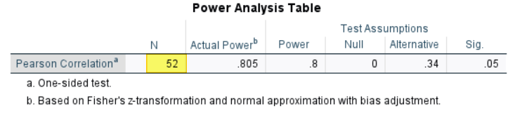
The SPSS Output Viewer will pop up with the results of your minimum sample size calculation. As you can see, the minimum sample size for our example Pearson correlation test is 52. If you don’t think that the minimum sample size calculated for your study is feasible, consider running the calculation again with different values.
***************
That’s it for this tutorial. You should now be able to calculate the minimum sample size for a Pearson correlation coefficient using SPSS power analysis.
***************