Fisher’s Exact Test in R

Fisher’s exact test is used to determine whether a relationship exists between two categorical variables, for example, students’ gender and their study mode (part-time, full-time).  This test is typically used as an alternative to the chi-square test of independence when sample sizes are small and the variables are dichotomous.

In this tutorial we will show you how to conduct and interpret Fisher’s exact test in R, and how to report the results in APA style.  As usual, we will work with RStudio, a program that makes it easier to work with R.

The Data

The data frame for a Fisher’s exact test must include two categorical variables.  If you haven’t already imported or created a data frame in R, we have tutorials on importing Excel, CSV and SPSS files into R, and another one on manually entering data in R.

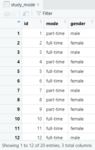
Our example data frame contains the categorical variables gender and mode for 20 fictitious college students.  You can see the first 12 records in the screenshot below.  We want to determine whether there is a relationship between students’ gender and their study mode (part-time or full-time).

Creating a Contingency Table

If your data form is formatted such that each column represents one of your variables and each row represents one of your subjects, it is important to create a contingency table of your two variables before you conduct Fisher’s exact test in R.

Contingency tables summarize the relationship between categorical variables.  Each row of the table represents one group of one of the variables (e.g., the female group of gender).  Each column represents one group of the other variable (e.g., the full-time group of mode).  The frequency for the particular combination of groups (e.g., females who study full-time) appears in the table cells.

We use the following command to create a contingency table for two variables in R:

contingencytable <- xtabs ( ~ x + y, data = dataframe)
contingencytable

Replace the highlighted text above as follows:

• contingencytable: the name you assign to your contingency table in R.  Feel free to use another name if it is more meaningful to you.
• dataframe: the data frame that contains your two categorical variables (the data frame for our example is study_mode)
• x and y: the names of the two categorical variables (gender and mode in our example).  It doesn’t matter which variable is x and which is y.

For our example, the command is:

contingencytable <- xtabs ( ~ gender + mode, data = study_mode)
contingencytable

Here is a screenshot of our contingency table:

We cannot draw any firm conclusions from this contingency table alone.  We need to perform a statistical test to determine whether this distribution of frequencies means that there is any association between gender and study-mode.  Our first thought might be to conduct a chi-square test of independence, but this isn’t appropriate if your data violates any of the assumptions of that test.

When to Use Fisher’s Exact Test

Fisher’s exact test is typically used instead of the chi-square test of independence, when we have small samples, especially when the expected frequency of one or more of the cells of our contingency table is less than five.  Usually, Fisher’s exact test is performed on 2 x 2 contingency tables, that is, when we are working with two dichotomous variables, however it can also be used with larger tables.

We know that we have a fairly small sample (20 students) and that we are working with a 2 x 2 contingency table (both gender and study mode are dichotomous in our example).  Let’s generate a contingency table of expected frequencies to see whether any of the cells have a value of less than five. 

We can do this as follows:

chisq.test(contingencytable)$expected

We can see that the frequencies for two of the cells in our table are less than five, so our data violates one of the assumptions of the chi-square test of independence.  R also gives us a warning message saying:  ‘Chi-squared approximation may be incorrect‘.  Now that we know that our data violates one of the assumptions of the chi-square test, we can consider whether our data meets the assumptions of Fisher’s exact test.

Assumptions of Fisher’s Exact Test

In addition to considerations of sample size and expected values in contingency tables, the assumptions of Fisher’s exact test are:

• Both variables are categorical. Categorical variables include, for example, gender, nationality, and yes/no responses.

• The groups in each of your categorical variables are mutually exclusive. For example, students’ mode of study cannot be both part-time and full-time.

• Independence of observations. None of the observations in the data set is influenced by any of the other observations.

Fisher’s Exact Test in R

We use the following command to conduct Fisher’s exact test in R.  

fisher.test(contingencytable)

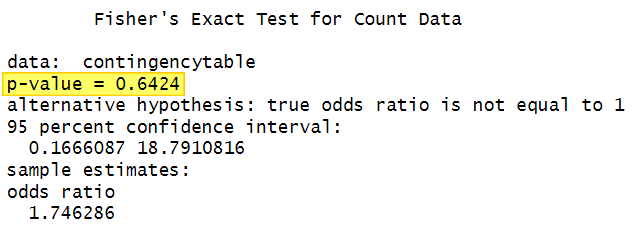
The results of the test for our example are presented below:

Interpreting Fisher’s Exact Test Results in R

The p value is the most important value that we see in the R output for Fisher’s exact test (highlighted in the screenshot above).

If the p value is less than equal to the alpha level we have selected for our test, we conclude that there is a significant association between our two variables.  An alpha level of .01 or .05 is typical.

However, if the p value is greater than the alpha level we selected for the test, then we conclude there is not a significant association between our two variables.  Our p value of 0.6424 is greater than our selected alpha level of .05, so we conclude that there is no association between students’ gender and their study mode.

Reporting Fisher’s Exact Test in R

We can report the results Fisher’s exact test in APA Style like this: