One-Way ANOVA in R: A Step-by-Step Guide

We use the one-way analysis of variance (ANOVA) to assess whether there are significant differences in the means of a continuous dependent variable across three or more independent groups. For example, we could use this test to determine whether there are significant differences in the mean Research Methods exam scores of students in three different college majors.

In this tutorial, we will show you how to perform and interpret a one-way ANOVA in R, how to conduct a post-hoc test, and how to report the results in APA style. As with our other R tutorials, we will be using RStudio, a program that makes it easier to work with R.

The Data

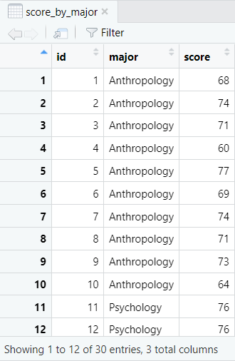
We start from the assumption that you have already created a data frame in R, or imported your data from another application like Excel, CSV or SPSS. The data frame for a one-way ANOVA needs to include a continuous dependent variable and an independent grouping variable.  Our example contains the Research Methods exam scores from a sample of 30 fictitious students enrolled in one of three college majors – Anthropology, Psychology or Sociology.   The first 12 records are illustrated below:

Our continuous dependent variable is Research Methods exam scores and our independent grouping variable is college major.  We want to know whether there are significant differences between mean Research Methods exam scores based on students’ major.  

One-Way ANOVA Assumptions

The assumptions of the one-way ANOVA are as a follows:

• Independence of observations. None of the observations in your data frame are influenced by any of the other observations.
• Absence of extreme outliers.  There should be no extreme outliers in your dependent variable (e.g., exam scores) for any of your groups (e.g., college majors). We will explain how to test this assumption with a boxplot in R.
• Normal distribution. The dependent variable (e.g., exam scores) should be approximately normally distributed for each of your groups (e.g., college majors). We will show you how to test this assumption in R using the Shapiro-Wilk test by group.
• Equal variances. The variance for the dependent variable (e.g., exam scores) should be approximately equal for each of your groups (e.g., college majors).  We will show you how to test this assumption by computing Levene’s test in R.

Testing the One-Way ANOVA Assumptions in R

While the independence of observations assumption refers to the way in which the study is designed, the other three assumptions can be tested in R. Throughout this tutorial, the commands we use in R are typed in blue text.  Lines of pink text starting with # provide explanations of these commands. R will ignore anything on lines that start with #.

Testing the Absence of Extreme Outliers Assumption

We can test this assumption by visualizing our dependent variable for each group of our independent variable with a boxplot:

# Install the ggplot2 visualization package if you don’t have it installed on your device install.packages("ggplot2")

# Load the ggplot2 package  
library(ggplot2) 

# Create boxplots of the dependent variable for each group of your independent variable
ggplot(dataframe, aes(x = groupingvariable, y = dependentvariable, fill = groupingvariable)) + geom_boxplot() + labs(title = "Title")

You will need to replace the highlighted text to create your grouped boxplots as follows:

• dataframe: the name of your data frame (score_by_major in our example).
• groupingvariable: the name of your grouping variable (major in our example). This variable appears twice in the above command
• dependentvariable: the name of your continuous dependent variable (score in our example).
• Title: this is optional. We want to add the title Research Methods Exam Scores by Student Major  

So, for our example, we use the following command:

# Create boxplots score grouped by major (our example)
ggplot(score_by_major, aes(x = major, y = score, fill = major)) + geom_boxplot() + labs(title = "Research Methods Exam Scores by Student Major")

R displays boxplots in the Plots tab of the bottom right panel of RStudio.  Our boxplots are below.

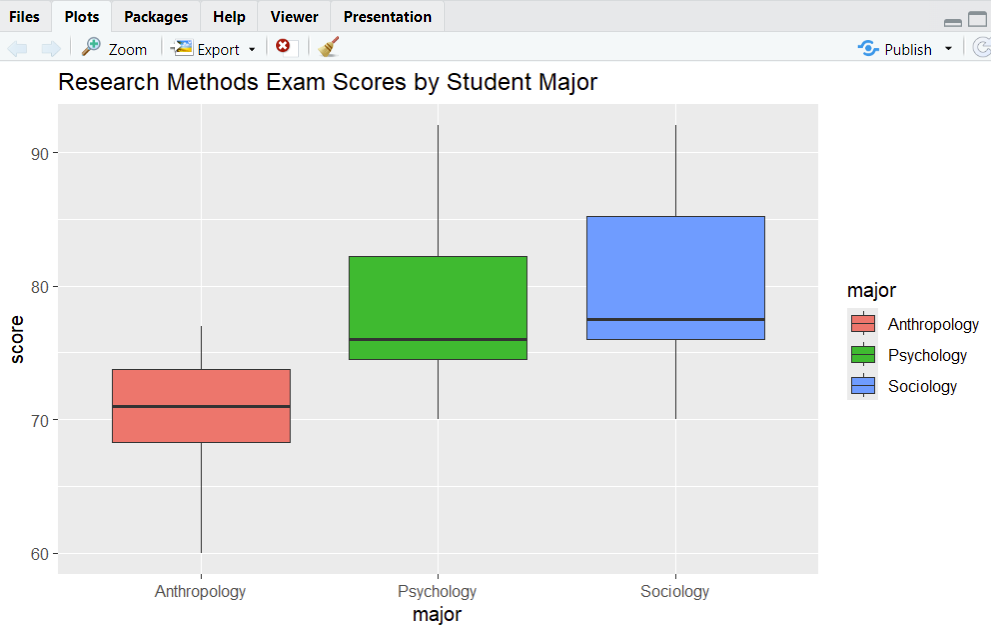
We can see that there are no outliers for Research Methods exam scores for any of the majors, so our data satisfies this assumption.  For reference, by default, R uses black dots to represent outliers, as illustrated below.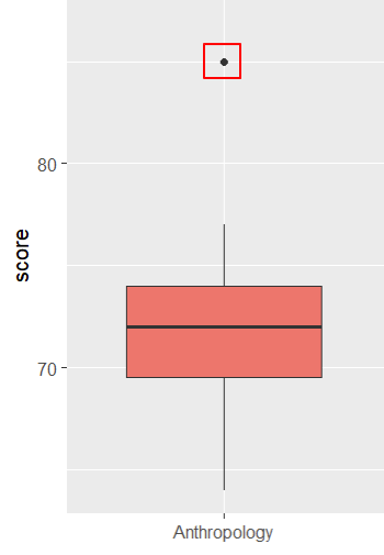

Testing the Normal Distribution Assumption

We can test the normal distribution assumption by computing the Shapiro-Wilk test by group:

# Compute Shapiro-Wilk test of a dependent variable by group
with(dataframe, shapiro.test(dependentvariable[groupingvariable == "group"]))

Replace the highlighted text as below:

• dataframe: your data frame (score_by_major in our example).
• dependentvariable: the variable in this data frame that you are testing for normality by group (score in our example).
• grouping variable: the variable you are using to group the dependent variable (major in our example).
• group: the group of this grouping variable that you are using for your normality test (we need to run the command once each for the Anthropology, Psychology and Sociology groups)

So, to compute the Shapiro-Wilk test for score by major, we type the following into the RStudio console:

# Compute Shapiro-Wilk test for score by Anthropology major
with(score_by_major, shapiro.test(score[major == "Anthropology"]))

# Compute Shapiro-Wilk test for score by Psychology major
with(score_by_major, shapiro.test(score[major == "Psychology"]))

# Compute Shapiro-Wilk test for score by Sociology major
with(score_by_major, shapiro.test(score[major == "Sociology"]))

Here are the results of our Shapiro-Wilk tests:

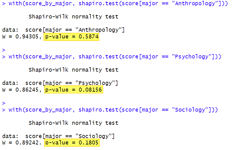
With a Shapiro-Wilk test, what you want to see are p values that are greater than .05 as is the case with each of our majors.  With these p values, we can assume that the score for each of our majors is normally distributed.

If, however, you have p values that are less than or equal to .05, you can not assume that the data is normally distributed.

Testing the Equal Variances Assumption

We can test the equal variances assumption using Levene’s test:

# Install the car package if it isn’t installed on your device
install.packages("car")

# Load the car package  
library(car) 

# Compute Levene’s test
leveneTest(dependentvariable ~ groupingvariable, data = dataframe)

Replace the highlighted text above as follows:

• dependentvariable: the continuous dependent variable for which you are computing Levene’s test (score in our example)
• groupingvariable: the variable that you are using to group the above variable (major in our example)
• dataframe: the data frame that contains both of these variables (score_by_major in our example)

So, for our example, we have the following:

# Compute Levene’s test for our example
leveneTest(score ~ major, data = score_by_major)

The results of Levene’s test for our example are below:

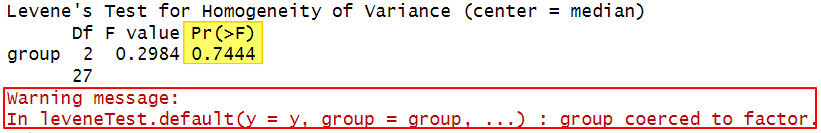
There are two things to note here. Firstly, if your grouping variable isn’t coded as a factor in R, you may receive a warning message stating: "In leveneTest.default(y = y, group = group, …) : group coerced to factor" (outlined in red above).  You can disregard this message if the variable in question is a grouping variable (like major in our example).

Secondly, if the p value (highlighted in yellow above) is greater than .05 (as is the case with our p value of 0.7444 ), then your data satisfies the equal variances assumption. If this p value is less than or equal to .05, this assumption is not satisfied.

Performing the One-Way ANOVA in R

Before we perform the one-Way ANOVA, we want to generate some descriptive statistics, specifically, the count, mean and standard deviation of our continuous dependent variable by group.

Descriptive Statistics

The most straightforward way to generate these descriptive statistics is as follows:

# Count the number of cases of your dependent variable by group
aggregate(dataframe$dependentvariable, list(dataframe$groupingvariable), FUN=length)

# Compute the mean of your dependent variable by group
aggregate(dataframe$dependentvariable, list(dataframe$groupingvariable), FUN=mean)

# Compute the standard deviation of your dependent variable by group
aggregate(dataframe$dependentvariable, list(dataframe$groupingvariable), FUN=sd)

As above, we replace the highlighted text as follows:

• dependentvariable: your continuous dependent variable (score in our example)
• groupingvariable: the variable that you are using to group this variable (major in our example)
• dataframe: the data frame that contains these two variables (score_by_major in our example)

So, for our example, we type the following into the RStudio console:

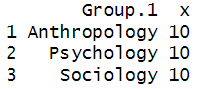
# Compute the number of scores for each major
aggregate(score_by_major$score, list(score_by_major$major), FUN=length)

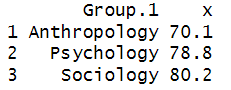
# Compute the mean score for each major
aggregate(score_by_major$score, list(score_by_major$major), FUN=mean)

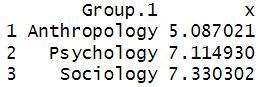
# Compute the standard deviation for each major
aggregate(score_by_major$score, list(score_by_major$major), FUN=sd)

Our results are presented below:

Counts	Means	Standard Deviations

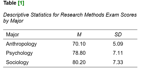
We can see that students in the Sociology major received the highest mean scores, followed by those in the Psychology major.  The students in the Anthropology major received the lowest mean scores.

Our means are displayed to one decimal place only because the next digit for all of them is 0 (70.10, 78.80 and 80.20, respectively).  You may see a larger number of decimal places for your own example.

The One-Way ANOVA

Once we have ensured that our data meet the test assumptions and generated descriptive statistics, it is time to perform the one-way ANOVA itself.

# Perform one-way ANOVA
myanova <- aov(dependentvariable ~ groupingvariable, data = dataframe)

# View your one-way ANOVA model
summary (myanova)

You should replace the highlighted text above as follows:

• myanova: this is the name that we have used for our ANOVA model. We will use it throughout this tutorial, but you can use a different name here.
• dependentvariable: your dependent variable (e.g., score)
• groupingvariable: your grouping variable (e.g., major)
• dataframe: the data frame containing the above variables (e.g., score_by_major)

Let’s see how this looks for our example:

# Perform one-way ANOVA to determine whether there are significant differences in mean exam scores based on students’ major
myanova <- aov(score ~ major, data = score_by_major)

# View the output of the above one-way ANOVA
summary (myanova)

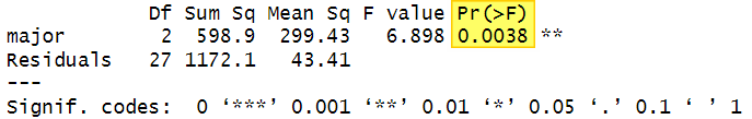
The output for our one-way ANOVA is as follows:

Interpreting The Results of the One-Way ANOVA

If your p value is less than or equal to the alpha level you set for your test, then there is a significant difference between the means of your groups.  Our p value of 0.0038 is less than our selected alpha level of .05, indicating that there is a significant difference between the mean Research Methods exam scores of students in different college majors.  

However, the ANOVA doesn’t tell us which mean(s) are significantly different from which other mean(s). To find out where the difference(s) lie, we need to conduct a post hoc test.

Post-Hoc Testing

One of the most common post-hoc tests that researchers conduct after a significant one-way ANOVA is Tukey’s honestly significant difference (HSD) test.  We can compute this test in R as follows:

# Compute Tukey’s HSD
TukeyHSD(myanova)

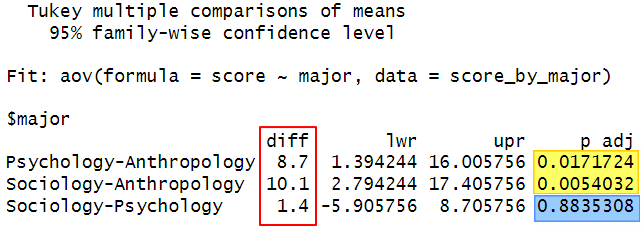
The values in the “diff” column tell us the difference in the mean Research Methods exam scores for each pair of majors.  If the p value in the “p adj” column is less than .05, then this difference is significant at the .05 alpha level.  We can see that there is a significant difference for both (a) the Psychology-Anthropology and (b) the Sociology-Anthropology pairs.  On the other hand, the p value for the Sociology-Psychology pair is above .05 indicating that the difference between the mean scores for students in these majors is not significant.

Reporting a One-Way ANOVA

If we wanted to report the results of our one-way ANOVA in APA Style, we could write something like this:

***************

That’s it for this tutorial.  You should now be able to perform and interpret a one-way-ANOVA in R, conduct a post-hoc test, and write up your results in APA style. 

***************