Paired Samples T-Test in R

In this tutorial, we will show you how to conduct and interpret a paired samples t-test in R, and how to report the results.

The paired samples t-test, also known as the dependent samples t-test, compares the mean difference between two measurements of the same continuous variable.  It is sometimes used in the context of a pre-test, post-test research design.  For example, we could record the body weight of dieters before and after they completed a  healthy food preparation program.

As with all of our R tutorials, we recommend working with RStudio, a program that makes it easier to work with R.

The Data

First of all, we need to import or create a data frame in R.  Please see our tutorials on importing your Excel, CSV and SPSS files into R, and our tutorial on manually entering data in R.

The data frame for a paired samples t-test should include two columns representing your paired continuous variables.  Each row should represent one participant. 

Our example data frame contains the body weight measurements (in lbs) of 20 participants both before they started a healthy food preparation program, and also after they completed this program.  We want to know whether there is a difference between these two body weight measurements.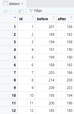

Paired Samples t-Test Assumptions

The assumptions of the paired samples t-test are as a follows:

• The observations within each group should be independent.
• There should be no significant outliers in the differences between the paired variables.  We will show you how to test this assumption with a boxplot.
• The differences between the paired variables should be approximately normally distributed.  We will show you how to test this assumption with a Shapiro-Wilks test.  It is worth noting, however, that the paired samples t-test is generally robust to minor violations of normality, especially with larger sample sizes (e.g., > 30).  

Testing Paired Samples t-Test Assumptions in R

It is important to note that the outliers and normality assumptions refer to the differences between the paired variables, rather than to the variables themselves.  That’s why we need to create a variable that represents these differences:

differences <- dataframe$x – dataframe$y

Replace the highlighted text in this command as follows:

• dataframe: the name of the data frame that contains your paired variables (dieters in our example)
• x: the name of the variable that represents the first set of measurements (before in our example)
• y: the name of the variable that represents the second set of measurements (after in our example)

For our example, the command is as follows:

differences <- dieters$before – dieters$after

Once you select the enter key on your keyboard, you will see your this new differences variable in the Environment tab in the top right panel of RStudio: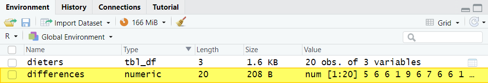

Testing the ‘No Significant Outliers’ Assumption

We can now test the outliers assumption by visualizing this differences variable with a boxplot. The easiest way to do this is as follows:

boxplot (differences)

Once we click the enter key on our keyboard, RStudio will display our boxplot in the Plots tab of the bottom right panel of RStudio.

Our example boxplot is displayed in the left column of the table below.  It does not have any outliers, so our data pass this assumption.  For comparison, the boxplot displayed in the right column has a noticeable outlier (we have drawn a red box around it).

Boxplot without outliers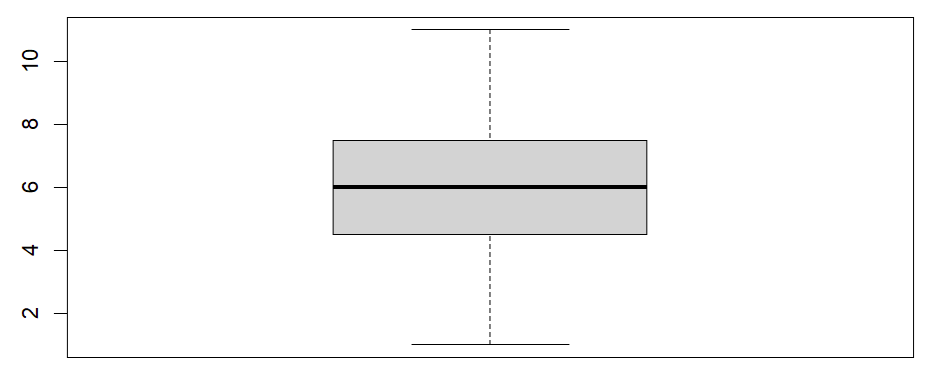

Boxplot with outlier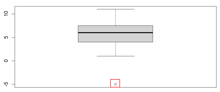

Testing the Normality Assumption

We can test the normality assumption using the Shapiro-Wilk test as follows:

shapiro.test (differences)

Here are the results of our Shapiro-Wilk test: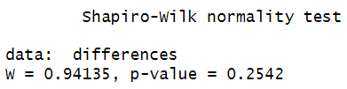

We assume normal distribution if the p value is greater than .05.  Our p value of 0.2542 is well above .05, so we assume that the differences between our paired variables are normally distributed.

When the p value is less than or equal to .05, however, we can not assume that the data is normally distributed.

The Paired Samples t-Test in R

Once you have ensured that your data meet the assumptions outlined above, you can use the following command to conduct the paired samples t-test itself:

t.test (dataframe$x, dataframe$y, paired = TRUE)

Replace the highlighted text with the relevant information for your study as follows:

• dataframe: the data frame that contains your paired variables (e.g., dieters).
• x: the variable that contains the first set of measurements (e.g., before)
• y: the variable that contains the second set of measurements (e.g., after)

So, for our example, we enter the following in the RStudio console:

t.test (dieters$before, dieters$after, paired = TRUE)

We also recommend computing the mean and the standard deviation of your paired variables since you would typically include this information when you report your results. 

You can compute the mean of a variable as follows:

mean (dataframe$variable)

You can compute the standard deviation of a variable as follows:

sd (dataframe$variable)

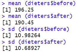
So, for our example, we type the following into the RStudio console:

mean (dieters$before)
mean (dieters$after)
sd (dieters$before)
sd (dieters$after)

The Results of the Paired Samples t-Test

The results of the paired samples t-test for our example are as follows: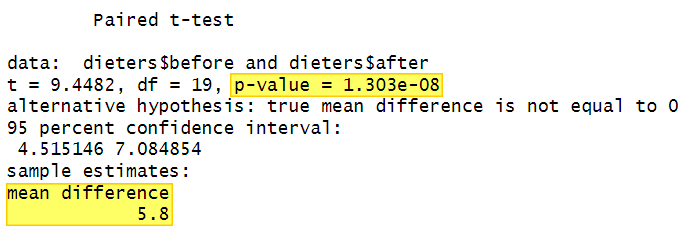

First, we note that there is a mean difference of 5.8 lbs between dieters’ body weight measurements before and after they complete the healthy food preparation program.  The fact that this is a positive number means that dieters’ mean body weight measurements were lower for the second measurement (after the program) than they were for the first measurement (before the program).  That is, they lost weight.  A negative mean difference would have meant that dieters’ second mean body weight measurements were higher than their first mean body weight measurements. 

The other important value from the paired samples t-test is the p value.   If the p value is less than or equal to the alpha level we have set for our test, then the difference between the paired measurements is significant.  Setting an alpha level of .05 or .01 is typical.  Our p value of 1.303e-08 converts to the real number 0.00000001303.  Since this is much less than our selected alpha level of .05, we conclude that the difference between dieters’ body weight measurements before and after the healthy food preparation program is significant.

On the other hand, if the p value is greater than our selected alpha level, we can not conclude that there is a significant difference between our paired measurements (dieters’ body weight in our example).

We also asked R to compute the means and standard deviations of our two variables:

Reporting a Paired Samples t-Test

If we wanted to report the results of our paired samples t-test in APA Style, we could do so as follows:

***************

That’s it for this tutorial.  You should now be able to conduct and interpret a paired samples t-test in R, and write up the results of your test. 

***************