It is an assumption of many statistical tests that our data be normally distributed. There are two broad approaches to testing normality. The first is to assess it visually, by reviewing a graph of the data. The second is to assess it numerically, by conducting a normality test.
In this quick tutorial, we will show you how to test for normality using both graphs and normality tests in R. We will work with RStudio, a program that makes it easier to work with R.
We start from the assumption that you have created or imported a data frame in R containing the variable(s) that you want to test for normality. Please see our tutorials on importing SPSS, Excel and CSV files into R, or our tutorial on manually entering data in R.
Visual Methods for Assessing Normality
One of the most common methods for assessing normality visually is the Q-Q plot, or Quantile-Quantile plot. If the data points on your Q-Q plot fall close to the straight diagonal line that runs from the bottom left to the top right corner of the plot, you can assume that your data is normally distributed.
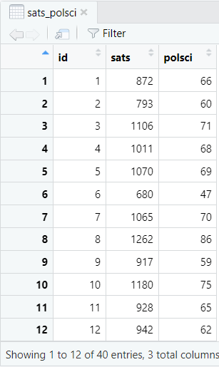
We want to determine whether the variable (vector) polsci in the data frame sats_polsci is normally distributed.
Enter the following command in the RStudio console and then select enter on your keyboard to create a Q-Q plot in R:
qqnorm(dataframe$variable, frame = FALSE)
qqline(dataframe$variable)
Replace the highlighted text with the data that you want to use to create your own Q-Q plot:
- dataframe: the name of your data frame in RStudio. The example that we are using is sats_polsci
- variable: the variable (vector) in the above data frame that you want to test for normality. In our example this is polsci
The command that we use to generate the Q-Q plot for our example is:
qqnorm(sats_polsci$polsci, frame = FALSE)
qqline(sats_polsci$polsci)
Click the enter key on your keyboard. You will see your Q-Q Plot in the Plots tab of the bottom right panel of RStudio.
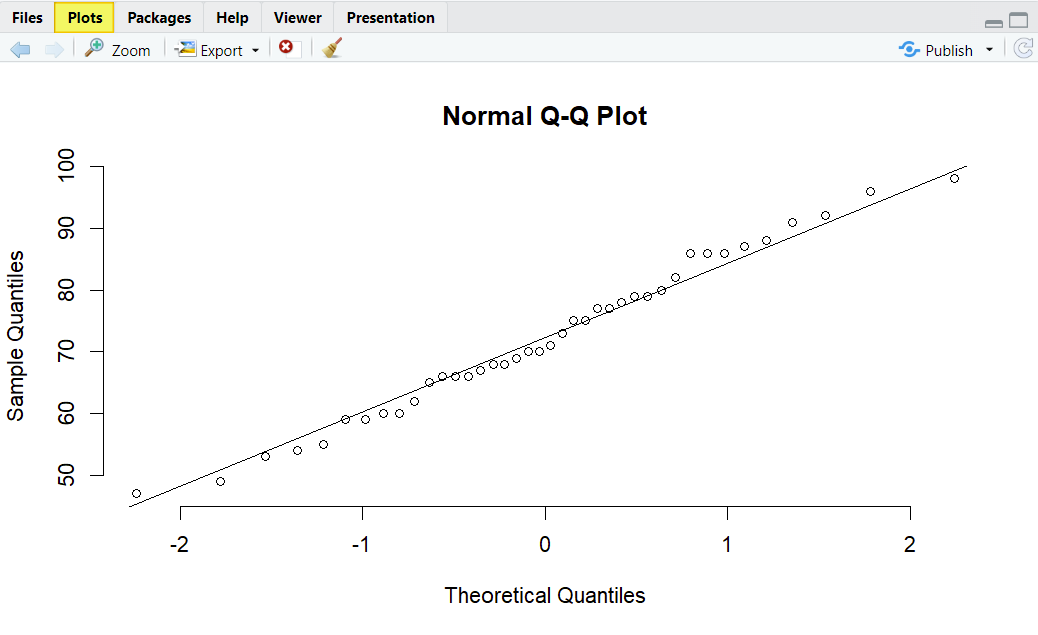
We can see that the data points fall close to the diagonal line. Therefore, we can conclude that our data is normally distributed.
Numerical Tests for Assessing Normality
It is a good idea to combine your Q-Q plot with a numerical test for normality such as the Shapiro-Wilk test or the Kolmogorov-Smirnov test. The Shapiro-Wilk test is usually recommended for smaller sample sizes (< 50), like our example.
Shapiro-Wilk Test for a Variable
To compute the Shapiro-Wilk test for a variable, enter the following command in the RStudio console and then select enter on your keyboard:
shapiro.test(dataframe$variable)
Replace the highlighted text with the information about the variable that you want to test for normality as follows:
- dataframe: the name of your data frame in RStudio (sats_polsci for our example)
- variable: the variable (vector) in the above data frame that you want to test for normality (polsci for our example).
So, this is what we enter to compute the Shapiro-Wilk test for our variable:
shapiro.test(sats_polsci$polsci)
The results of our Shapiro-Wilk test are as follows:
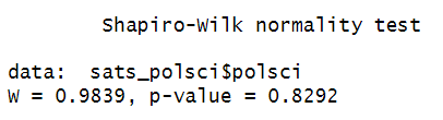
If the p value is greater than .05, then we can assume that the data is normally distributed. The p value for our test is 0.8292, so we assume that our variable is normally distributed.
If, however, the p value is less than or equal to .05, we assume that the data is not normally distributed.
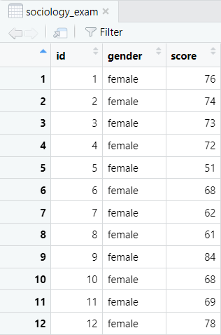
Shapiro-Wilk Test by Group
We can also compute the Shapiro-Wilk test for groups of a variable. For example, we want to determine whether the score variable in the data frame below is normally distributed for both levels of the gender variable (males and females).
To compute the Shapiro-Wilk test for groups of a variable, we can use the following command:
with(dataframe, shapiro.test(variable[groupingvariable == "group"]))
Replace the highlighted text above as follows:
- dataframe: the name of your data frame (e.g., sociology_exam)
- variable: the variable (vector) in this data frame that you want to test for normality by group (e.g., score)
- grouping variable: the variable (vector) you want to use to group the above variable (e.g., gender)
- group: the group or level of the grouping variable that you want to use for your normality test (we will run the command once for the male group and once for the female group)
So, this is what we type to compute the Shapiro-Wilk test for the score variable by the gender grouping variable:
with(sociology_exam, shapiro.test(score[gender == "male"]))
with(sociology_exam, shapiro.test(score[gender == "female"]))
The results of our Shapiro-Wilk test by group are:
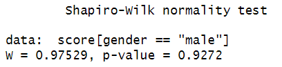
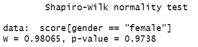
The p value of the Shapiro-Wilk test for male students is 0.9272. Since this is greater than .05, we assume that the score variable is normally distributed for male students. Similarly, the p value of 0.9738 for female students is greater than .05, so we also assume that the score variable is normally distributed for female students.
***************
That’s it for this tutorial. You should now be able to test data for normality in R using the Q-Q plot and the Shapiro-Wilk test.
***************